Probability Calibration in ML
Background
When are the outputs of predict_proba actual probabilities? If the model says \(0.9\), should I assume that among all the cases it scored \(0.9\), roughly \(90\%\) were positive. Not always!
For a logistic regression that reflex is mostly harmless. For a random forest, it can be badly wrong. The failure is silent, because the model’s accuracy and AUC look perfectly fine while the numbers themselves lie.
That is what calibration is about: whether a predicted probability means what it says. A model can rank cases beautifully (every positive scored above every negative) and still be dangerously miscalibrated, systematically over- or under-stating its confidence. Ranking and calibration are different, and most of machine learning optimizes for the first while quietly assuming the second.
This blog post is a deep dive on calibration in ML models. Calibration is not free, it is not always necessary, and applying it blindly can cost you. So I will walk through when the number actually needs to mean something, how to tell whether it does, and how to fix it when it doesn’t.
Notation
Consider binary classification with label \(Y \in \{0, 1\}\) and a model that outputs a score \(\hat{p}(X) \in [0, 1]\) meant to estimate \(P(Y = 1 \mid X)\). The model is perfectly calibrated if
\[ P\big(Y = 1 \mid \hat{p}(X) = p\big) = p \quad \text{for all } p \in [0, 1]. \]
In words: of all the cases assigned score \(p\), a fraction \(p\) are truly positive. This is a property of the score’s marginal relationship to the outcome, not of individual predictions — which is why a model can be calibrated and useless (predict the base rate for everyone) or sharp and miscalibrated (rank perfectly, wrong magnitudes). Good probabilities need both calibration and resolution (the tendency to push scores away from the base rate toward \(0\) and \(1\)).
A Closer Look
When you actually need it
The single most useful question is: does a downstream decision depend on the magnitude of the probability, or only on its order?
If you only need to rank — show the top-\(k\) most likely churners, sort leads by score, compute AUC — calibration is irrelevant. Any monotonic transform of the score leaves the ranking, and hence AUC, unchanged. Recalibrating buys you nothing here and, with isotonic regression, can even hurt by introducing ties.
Calibration starts to matter the moment a probability feeds arithmetic. Expected-value decisions (\(\text{value} = p \cdot \text{gain} - (1-p) \cdot \text{cost}\)) need the \(p\) to be right, not just ordered. Thresholding at a fixed operating point (act when \(p > 0.7\)) assumes \(0.7\) means something. Combining model outputs with other probabilities, feeding them to a Bayesian update, or reporting them to a human who will treat \(0.9\) as “nearly certain” — all of these break under miscalibration. This is closely related to the distinction I drew between causal and predictive models: the use case dictates which properties of the output you are allowed to trust.
Diagnosing miscalibration
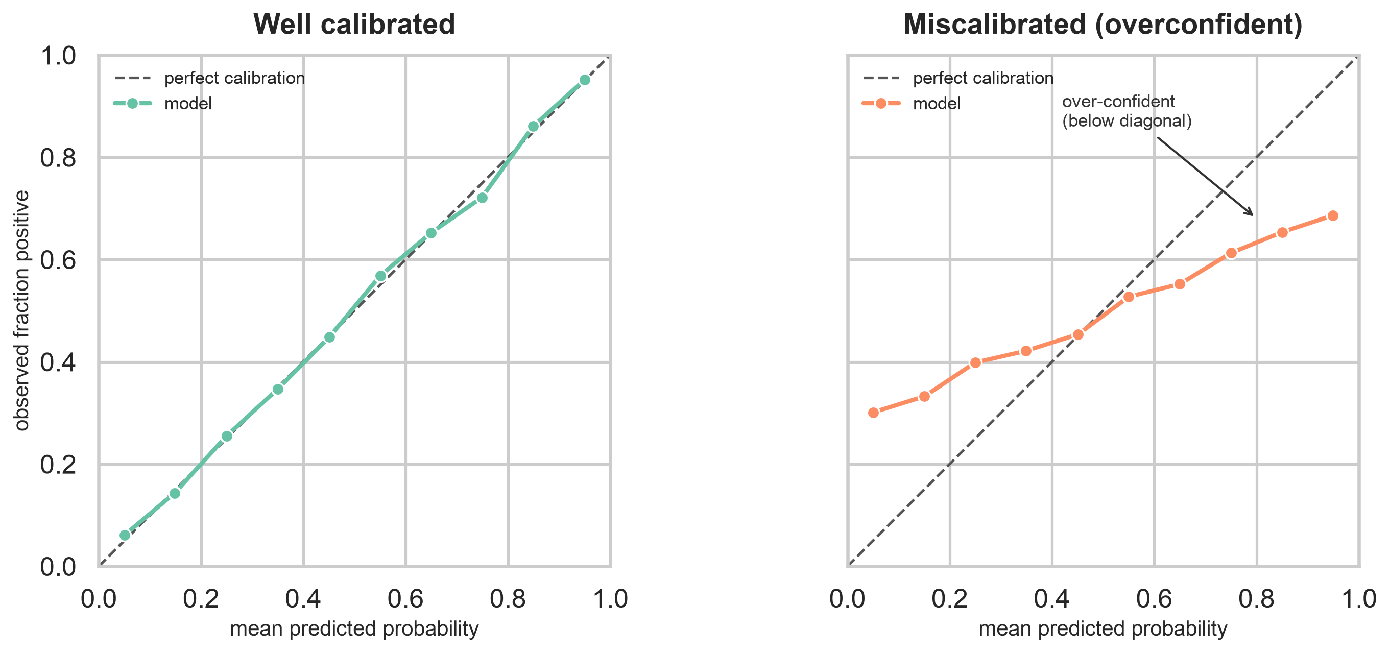
The workhorse diagnostic is the reliability diagram: bin predictions by score, and for each bin plot the mean predicted probability (\(x\)-axis) against the observed fraction of positives (\(y\)-axis). Perfect calibration lies on the \(45^\circ\) line. Curves below the diagonal signal over-confidence; curves above it, under-confidence. It is one of the plots I think everyone should have in their back pocket.
The two panels below show the contrast. On the left, a well-calibrated model hugs the diagonal — its stated probabilities match observed frequencies. On the right, an over-confident model: it sits above the diagonal for low scores and below it for high ones, the telltale crossing pattern of a classifier whose probabilities are pushed too hard toward the extremes.
For a single number, use a proper scoring rule—a loss function that is minimized if and only if the predicted probability equals the true probability. The Brier score is the most intuitive: it is simply the mean squared error of the probabilities,
\[ \text{Brier} = \frac{1}{n} \sum_{i=1}^{n} \big(\hat{p}_i - y_i\big)^2, \]
and log loss is its logarithmic cousin. But mind the trap: a low Brier score does not guarantee good calibration. According to Murphy’s decomposition, the Brier score is a sum of reliability (calibration), resolution (how much the predictions differ from the base rate), and an inherent uncertainty term.
A model that is “sharp” but miscalibrated—one that confidently predicts \(0.9\) for a group that is actually \(70%\) positive—can still achieve a lower Brier score than a perfectly calibrated model that conservatively predicts \(0.7\) for everyone. In other words, better discrimination can mask poor calibration in a single aggregate metric. To know if your probabilities are actually trustworthy, you cannot rely on the Brier score alone; pair it with a reliability diagram.
Miscalibration varies by model
Not all classifiers misbehave the same way. Logistic regression is typically well-calibrated out of the box: minimizing log loss with the canonical logit link enforces a balance property that ties predicted probabilities to observed frequencies.
Naive Bayes, on the other hand, is over-confident — its independence assumption compounds evidence it should not, pushing scores toward \(0\) and \(1\).
Random forests and bagged ensembles, while extremely popular, are under-confident: averaging many trees pulls probabilities toward the middle, since it is rare for all trees to agree at the extremes, producing a telltale sigmoid reliability curve.
Max-margin methods like SVMs distort further still, because they optimize the decision boundary and never really estimate probabilities at all. Knowing the direction of a model’s bias tells you which fix will suit it.
Fixes
Calibration is a post-processing step: fit a monotonic map from raw scores to calibrated probabilities on held-out data. The two classic choices trade flexibility against data hunger.
Platt scaling
Platt (sigmoid) scaling fits a one-parameter logistic curve, \[\hat{p} = 1 / (1 + \exp(A f + B)),\] mapping the raw score \(f\) to a probability via just two fitted numbers \(A, B\). In practice, take the model’s held-out scores \(f_i\) and labels \(y_i\), then choose \(A\) and \(B\) by minimizing binary log loss for the calibrated probabilities. Once fitted, the same sigmoid map is applied to future raw scores; \(A\) controls the curve’s slope and \(B\) shifts it left or right. It is stable on small samples and ideal for the sigmoid-shaped distortion of under-confident models like random forests — but its rigid parametric shape cannot fix non-sigmoid errors.
Isotonic regression
Isotonic regression fits an arbitrary non-decreasing step function by least squares subject to monotonicity. In practice, take the model’s held-out scores \(f_i\) and labels \(y_i\), then estimate a monotone function \(g\) by solving \[ \hat g = \arg\min_{g \ \mathrm{nondecreasing}} \sum_i \big(y_i - g(f_i)\big)^2. \] The calibrated probability is then \(\hat p_i = \hat g(f_i)\). It corrects any monotonic distortion and is more powerful, but it overfits on small datasets and needs a few thousand calibration points to behave.
Temperature scaling
For multiclass neural networks, temperature scaling (dividing the logits by a single learned scalar \(T\) before the softmax) is the standard lightweight fix; it sharpens or softens all probabilities at once without changing the predicted class, so accuracy is untouched.
What Not to Do
The one thing you must not do is calibrate on the data the model trained on. An overfit classifier looks perfectly calibrated on its own training set, so the calibrator learns nothing and you ship overconfidence. Scikit-learn’s CalibratedClassifierCV handles this with cross-validation: it fits the calibrator on out-of-fold predictions, keeping calibration data disjoint from training data.
Bottom Line
- Calibration asks whether a predicted probability means what it says; a model can rank perfectly and still be badly miscalibrated.
- If you only need ranking or the argmax class, skip calibration — it changes nothing and can add noise.
- Calibrate when magnitudes drive decisions: expected value, fixed thresholds, probability arithmetic, or numbers shown to humans.
- Diagnose with a reliability diagram, not a Brier score alone — a proper scoring rule mixes calibration with discrimination.
- Fit the calibrator on held-out data: sigmoid for small samples and sigmoid-shaped error, isotonic when you have thousands of points, temperature scaling for neural nets.
Where to Learn More
For a hands-on tour, the scikit-learn calibration guide is excellent. For a deeper dive, see the references below.
References
Guo, C., Pleiss, G., Sun, Y., & Weinberger, K. Q. (2017). On Calibration of Modern Neural Networks. Proceedings of the 34th International Conference on Machine Learning (ICML), 1321–1330.
Niculescu-Mizil, A., & Caruana, R. (2005). Predicting Good Probabilities with Supervised Learning. Proceedings of the 22nd International Conference on Machine Learning (ICML), 625–632.
Platt, J. (1999). Probabilistic Outputs for Support Vector Machines and Comparisons to Regularized Likelihood Methods. In Advances in Large Margin Classifiers, MIT Press, 61–74.
Zadrozny, B., & Elkan, C. (2002). Transforming Classifier Scores into Accurate Multiclass Probability Estimates. Proceedings of the 8th ACM SIGKDD International Conference on Knowledge Discovery and Data Mining, 694–699.