Generating Variables with Predefined Correlation
Background
Suppose you are working on a project where the relationship between two variables is influenced by an unobserved confounder, and you want to simulate data that reflects this dependency. Standard random number generators often assume independence between variables, making them unsuitable for this task. Instead, you need a method to introduce specific correlations into your data generation process.
A powerful and efficient way to achieve this is through Cholesky decomposition. By decomposing a correlation matrix into its triangular components, you can transform independent random variables into correlated ones. This approach is versatile, efficient, and mathematically grounded, making it ideal for simulating realistic datasets with predefined (linear) relationships.
A Closer Look
The Algorithm
Assume we want to generate a vector \(Y\) with \(n\) observations and \(p\) variables with a target correlation matrix \(\Sigma\). The algorithm to obtain \(Y\) is as follows:
- Start with Independent Variables: Create a matrix \(X\) of dimensions \(n \times p\), where each column is independently drawn from \(N(0,1)\): \[ X = \begin{bmatrix}x_{11} & x_{12} & \cdots & x_{1p} \\x_{21} & x_{22} & \cdots & x_{2p} \\ \vdots & \vdots & \ddots & \vdots \\x_{n1} & x_{n2} & \cdots & x_{np}\end{bmatrix}. \]
- Decompose the Target Matrix: Perform Cholesky decomposition on the target correlation matrix \(\Sigma\) as: \[\Sigma = LL^T,\] where \(L\) is a lower triangular matrix.
- Transform the Independent Variables: Multiply the independent variable matrix \(X\) by \(L\) to obtain the correlated variables: \[Y = XL.\]
Here \(Y\) is an \(n\times p\) matrix where the columns have the desired correlation structure defined by \(\Sigma\). To ensure that \(\Sigma\) is a valid correlation matrix, it must be positive-definite. This condition guarantees the success of Cholesky decomposition and the correctness of the resulting correlated variables.
Mathematical Explanation
Let’s examine how and why this approach works. We know that \(\Sigma = LL^T\) and \(E(XX^T)=I\) by definition. We want to show that \(E(YY^T)=LL^T\). Here is the simplest way to get there:
\[\begin{align*} E(YY^T) &= E((LX)(LX)^T) \\ &= E(LXX^TL^T) \\ &= LE(XX^T)L^T \\ &= LL^T. \end{align*}\]
There you have it – the algorithm outlined above is mathematically grounded. The covariance matrix of \(Y\) is indeed equal to \(\Sigma\). Let’s now look at an example.
An Example
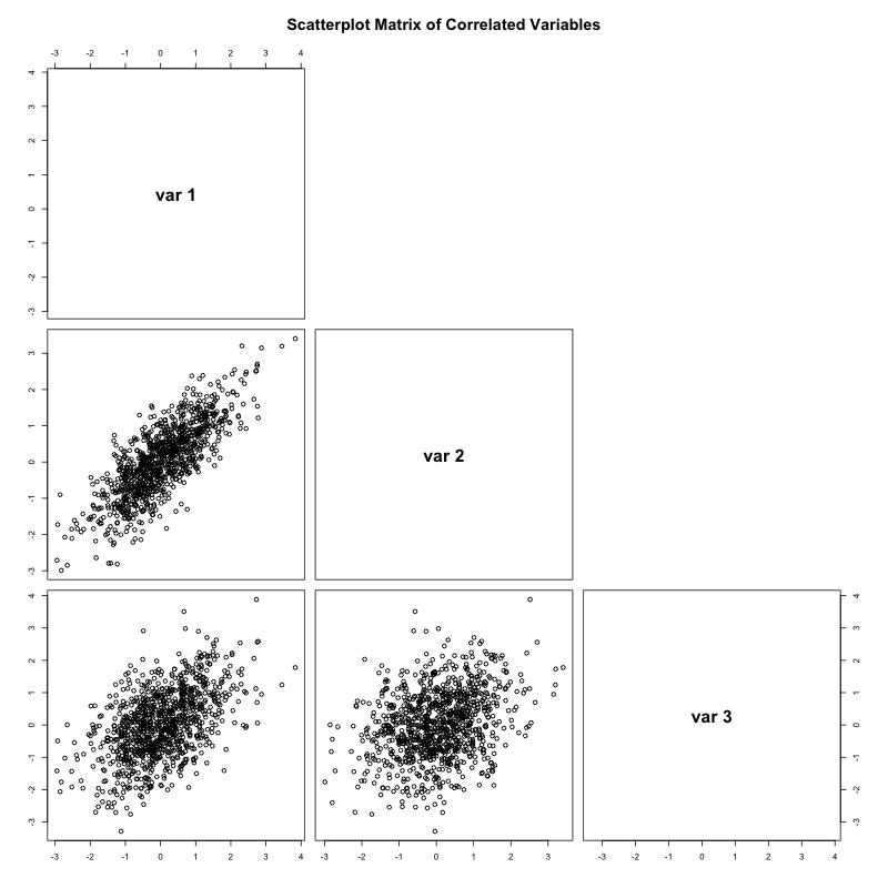
Let’s implement this in R and python with \(p=3\) and \(n=1,000\). Our target correlation matrix defines the desired relationships between the variables in \(Y\). In our example, we have pairwise correlations equal to \(0.8\) (b/w \(y_1\) and \(y_2\)), \(0.5\) (b/w \(y_1\) and \(y_3\)), and \(0.3\) (b/w \(y_2\) and \(y_3\)).
rm(list=ls())
set.seed(1988)

# Generate X, independent standard normal variables
n <- 1000
p <- 3
x <- matrix(rnorm(n * p), nrow = n, ncol = p)

# Define Sigma, the target correlation matrix
sigma <- matrix(c(
  1.0, 0.8, 0.5,
  0.8, 1.0, 0.3,
  0.5, 0.3, 1.0
), nrow = p, byrow = TRUE)

# Cholesky decomposition
L <- t(chol(sigma))
diag <- diag(c(1,1,1))
y <- t(diag %*% L %*% t(x))

# Print the results
print(cor(y))
          [,1]      [,2]      [,3]
[1,] 1.0000000 0.7875707 0.5111323
[2,] 0.7875707 1.0000000 0.3008518
[3,] 0.5111323 0.3008518 1.0000000
import numpy as np
np.random.seed(1988)
# Generate X, independent standard normal variables
n = 1000
p = 3
x = np.random.normal(size=(n, p))
# Define Sigma, the target correlation matrix
sigma = np.array([
[1.0, 0.8, 0.5],
[0.8, 1.0, 0.3],
[0.5, 0.3, 1.0]
])
# Cholesky decomposition
L = np.linalg.cholesky(sigma)
diag = np.diag([1, 1, 1])
y = (diag @ L @ x.T).T
# Print results
[[1. 0.78702913 0.48132289]
[0.78702913 1. 0.27758356]
[0.48132289 0.27758356 1. ]]Using our notation above we have:
\[\Sigma = \begin{bmatrix}1.0 & 0.8 & 0.5 \\0.8 & 1.0 & 0.3 \\ 0.5 & 0.3 &1.0\end{bmatrix}. \]
The chol function in R decomposes the matrix into a lower triangular matrix. In our example:
\[L^T = \begin{bmatrix}1 & 0.8 & 0.5 \\0 & 0.6 & -0.17 \\0 & 0.0 & 0.85 \end{bmatrix}. \]
Multiplying the independent variables \(X\) by the transpose of \(L\) ensures the output \(Y\) matches the specified correlation structure.
The cor function checks whether the generated data conforms to the target correlation matrix.
The two matrices match almost exactly. We can also visualize the three variables in a scatter plot matrix. Notice that higher correlation values (e.g., b/w \(y_1\) and \(y_2\)) correspond to stronger linear associations between them.
Bottom Line
A common data practitioner’s need is to generate variables with a predefined correlation structure.
Cholesky decomposition offers a powerful and efficient way to achieve this.