Double Descent for Statisticians
Background
Perhaps the first reflex a data scientist learns states a model that fits the training data perfectly has almost certainly overfit and will predict badly out of sample. The bias–variance trade-off draws a tidy \(U\) — too simple is biased, too flexible explodes the variance — and you aim for the sweet spot between. Interpolation is the cardinal sin.
Modern machine learning violates this reflex daily and gets away with it: enormous neural networks interpolate their training data yet generalize beautifully. Belkin et al. (2019) named the phenomenon double descent — push complexity past the interpolation point and out-of-sample error, after spiking, falls again, sometimes below the classical sweet spot. The bias–variance \(U\) is only the first half of the story.
Hastie, Montanari, Rosset, and Tibshirani (2022) show the whole phenomenon in the most classical model we have — linear least squares, no networks or kernels. They paint a story about interpolation, the geometry of the \(p > n\) regime, and above all about forgetting to regularize. Let’s take a closer look.
Notation
Take the usual linear model with i.i.d. data,
\[y_i = x_i^\top \beta + \varepsilon_i, \qquad \mathbb{E}(\varepsilon_i) = 0, \quad \text{Var}(\varepsilon_i) = \sigma^2,\]
with \(x_i \in \mathbb{R}^p\) and a design matrix \(X\) that is \(n \times p\). The single quantity that organizes everything is the overparametrization ratio
\[\gamma = p / n.\]
- when \(\gamma < 1\) the problem is underparametrized (more rows than columns, ordinary least squares applies);
- when \(\gamma > 1\) it is overparametrized and least squares no longer has a unique solution. In that regime the natural estimator is the minimum-norm, or ridgeless, least squares solution \[\hat\beta = (X^\top X)^+ X^\top y = X^+ y,\] the least-squares fit of smallest Euclidean norm, and equivalently the limit of ridge regression as the penalty vanishes, \(\hat\beta = \lim_{\lambda \to 0} \hat\beta_\lambda\).
Write the signal-to-noise ratio as \[\text{SNR} = \|\beta\|_2^2 / \sigma^2 = r^2/\sigma^2,\] and measure performance by the out-of-sample prediction risk at a fresh test point, \[R = \mathbb{E}\big[(x_0^\top \hat\beta - x_0^\top\beta)^2\big].\]
Lastly, we need the covariance matrix of the test point, \(\Sigma = \text{Cov}(x_0)\).
A Closer Look
The curve
Here is the whole phenomenon in one curve. It traces the out-of-sample risk of plain ridgeless least squares as the number of parameters grows relative to the sample size: the risk climbs as the model approaches just enough capacity to interpolate, blows up at that interpolation threshold, and then — against every classical instinct — falls a second time, eventually dipping below the null risk.
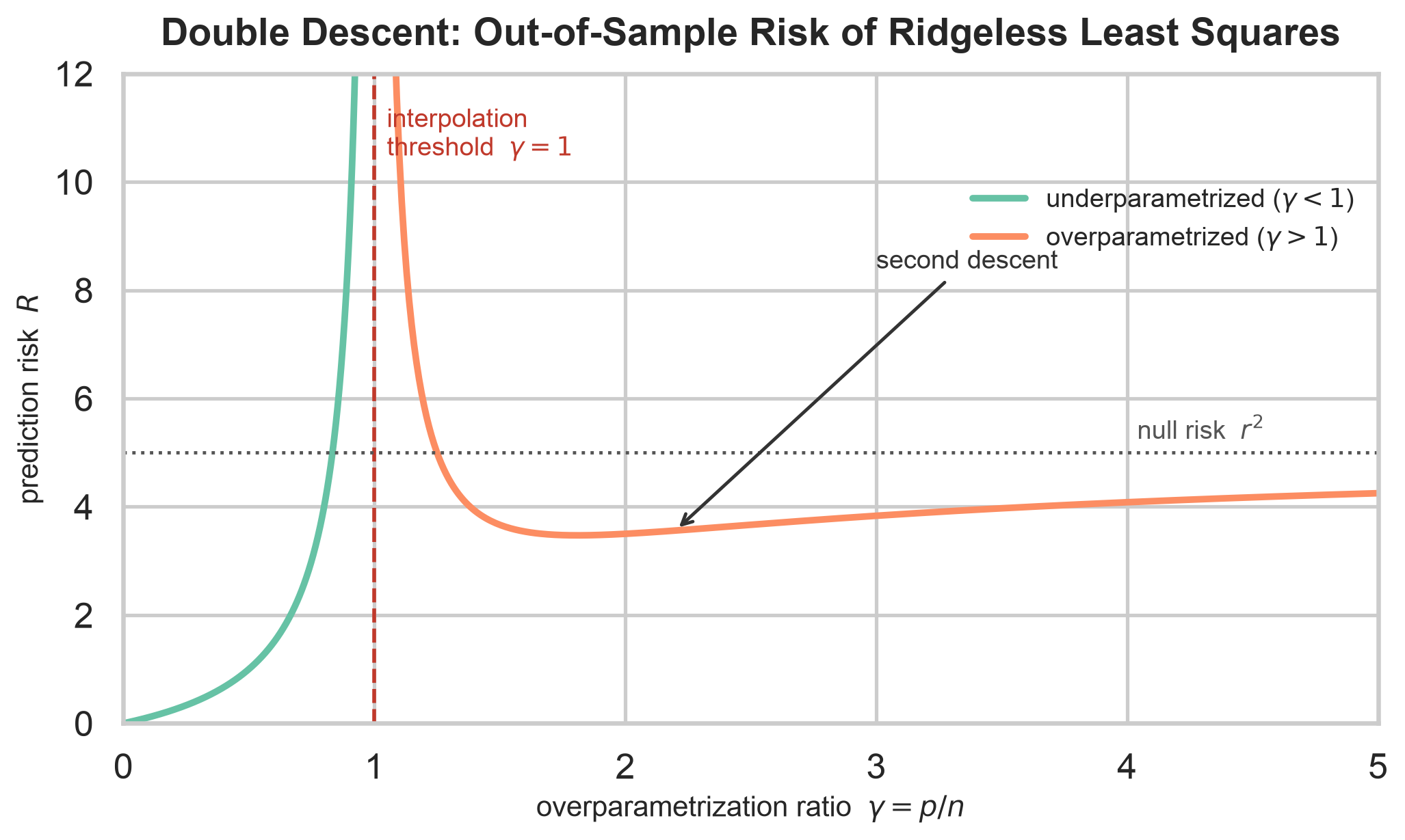
In math notation, we fix \(n\), sweep \(p\), fit ridgeless least squares at each step, and trace the out-of-sample risk against \(\gamma\) (isotropic case \(\Sigma = I\), signal norm \(\|\beta\|^2\) held fixed for a fair comparison). The risk climbs toward \(\gamma = 1\), blows up at the interpolation boundary, then descends a second time for \(\gamma > 1\).
Hastie et al. (2022) make this exact in the limit \(n, p \to \infty\) with \(p/n \to \gamma\):
\[ R \to \begin{cases} \sigma^2 \dfrac{\gamma}{1 - \gamma}, & \gamma < 1, \\[2ex] \underbrace{r^2\Big(1 - \tfrac{1}{\gamma}\Big)}_{\text{bias}} + \underbrace{\sigma^2 \dfrac{1}{\gamma - 1}}_{\text{variance}}, & \gamma > 1. \end{cases} \]
Below the boundary the risk is pure variance, diverging as \(\gamma \to 1\). Above it, a bias term grows with \(\gamma\) while a variance term shrinks — and that tension is the engine of the second descent.
Bias up, variance down
Why does the risk fall again past \(\gamma = 1\)? The two components move in opposite directions.
The bias rises with \(\gamma\) for a reason familiar from the \(p>n\) regime: the minimum-norm solution lives in the row space of \(X\), an \(n\)-dimensional slice of \(\mathbb{R}^p\). As \(p\) grows that slice shrinks relative to the whole, so more of \(\beta\) falls in the directions the data never see and the min-norm rule zeroes out. More parameters, more of \(\beta\) left on the table, more bias.
The variance falls with \(\gamma\), which feels backwards — surely more parameters means more variance? Not for the minimum-norm interpolator. Extra columns give the solver more directions to spread the fit across, so the minimum-norm solution to \(Xb = y\) generally has smaller norm as \(p\) grows, and a lower-norm interpolator is smoother and more stable — effectively more regularized, for free.
The spike at \(\gamma = 1\) is where both forces peak. With \(p \approx n\) the model has just barely enough capacity to interpolate and no slack to do it gracefully: \(X^\top X\) is nearly singular and the variance term \(\sigma^2/(\gamma-1)\) explodes. The interpolation threshold is not a sweet spot — it is the worst place to be.
It’s mostly a regularization story
The dramatic part of the curve (the divergence at \(\gamma = 1\)) is an artifact of insisting on interpolation, and interpolation is a choice, not a law. Ridgeless least squares is just ridge regression with the penalty dialed to zero, the one setting a statistician would never choose on purpose.
Hastie et al. (2022) prove it: optimally-tuned ridge dominates minimum-norm least squares at every \(\gamma\) and every SNR, well-specified or not. Its risk has no spike — proper \(\lambda\) smooths the curve into a single well-behaved descent, with the global minimum (under misspecification) sitting right around \(\gamma = 1\), exactly where ridgeless is worst. And the optimal penalty is estimable: leave-one-out cross-validation recovers it asymptotically.
Double descent is real and the math is beautiful, but the headline (more parameters fix overfitting) gets it backwards. The second descent just shows the minimum-norm interpolator picking up a hidden, growing dose of regularization as \(\gamma\) rises. You need not climb out to \(\gamma = 4\) to enjoy it; a ridge penalty and a cross-validation loop dial it in directly, skipping the peak entirely. Less “interpolation is secretly fine” than “under-regularization is bad, and overparametrization happens to re-regularize you on the way out.”
When overparametrization genuinely helps
That said, the strong claim — that the risk’s global minimum can live deep in the overparametrized regime — is true, but only under structure worth knowing.
In the isotropic, well-specified case it essentially never pays: even when \(\text{SNR} > 1\) creates a local minimum past \(\gamma = 1\), the global minimum stays underparametrized, and the risk only approaches the null risk \(r^2\) as \(\gamma \to \infty\). Overparametrization buys nothing you couldn’t get more cheaply.
Two things change the verdict.
Misspecification: if the truth has components your features cannot represent, adding features improves the approximation, and with enough signal the global minimum can cross the boundary.
Structure in the covariance: when \(\beta\) aligns with the leading eigenvectors of \(\Sigma\) — the “latent space” model, where each feature carries fresh information about a few latent drivers — the risk can fall monotonically across the whole overparametrized regime, bottoming out as \(\gamma \to \infty\). This is what large networks actually look like, and no accident: a linear model with a learned feature map is exactly the lazy-training (“neural tangent kernel”) linearization of an overparametrized network. Not an analogy — the same story.
Bottom Line
- Double descent needs no neural networks — plain ridgeless least squares shows it: the classical \(U\) for \(\gamma < 1\), a blow-up at the interpolation boundary \(\gamma = 1\), then a second descent for \(\gamma > 1\).
- Past the boundary, bias rises (min-norm \(\hat\beta\) is trapped in the row space) while variance falls (the interpolant smooths as \(p\) grows). The second descent is their tug-of-war.
- The peak at \(\gamma = 1\) is the worst place to be, not a sweet spot: \(X^\top X\) is near-singular and variance explodes.
- It is largely a regularization story: optimally-tuned ridge dominates ridgeless least squares everywhere and erases the spike, so tuning \(\lambda\) (e.g. by LOOCV) makes the drama disappear.
- Overparametrization wins globally only under structure — misspecification, high SNR, or \(\beta\) aligned with the top eigenvectors of \(\Sigma\).
References
Bartlett, P. L., Long, P. M., Lugosi, G., & Tsybakov, A. B. (2020). Benign overfitting in linear regression. Proceedings of the National Academy of Sciences, 117(48), 30063–30070.
Belkin, M., Hsu, D., Ma, S., & Mandal, S. (2019). Reconciling modern machine-learning practice and the classical bias–variance trade-off. Proceedings of the National Academy of Sciences, 116(32), 15849–15854.
Hastie, T., Montanari, A., Rosset, S., & Tibshirani, R. J. (2022). Surprises in high-dimensional ridgeless least squares interpolation. The Annals of Statistics, 50(2), 949–986.